Derivative Pricing and Valuation

A derivative is a financial instrument whose price is derived from one or more underlying assets. Thus, in very simple words, the price and value of a derivative stem from its underlying assets. The underlying assets can be anything that have some value. In the first part of this article, we will focus on the most common types of derivatives: forwards, futures, options, and swaps. In the second part, we will discuss more exotic derivatives. We will present not only the theory of derivative valuation, but also concrete examples in Python and Excel. Online version of the pricers can be found on our finance calculators page.

Although the pricing models differ for each type of derivative, the underlying principle is the same: financial derivatives are priced based on no-arbitrage principle, or the law of one price. For more details about financial theory and implementation of derivative valuation, see section Recommended Reading at the end of this article.

Forward Contracts

A forward contract is a private agreement between two parties giving the buyer an obligation to purchase an asset, and the seller an obligation to sell an asset at a set price at a future point in time. The underlying asset can be anything of value. In order to understand this better, let us look at a simple example.

READ OUR POSTS

Let us assume that the underlying asset here is a 10 kg bag of apples that have not been harvested yet. Technically, the underlying asset does not even exist, so it has no financial value. However, it is still possible to assign a price to it. Suppose that a farmer enters into a forward contract to sell the 10 kg bag of apples at a price of $20 in 3 months’ time when the apples will be harvested. The farmer does this because he fears that the price of apples may go down in the future, resulting in a loss for him. So in order to set off or hedge the potential loss, the farmer enters into a forward contract with a buyer who agrees to buy the 10 kg bag of apples at the $20 price determined today. This means that 3 months from now, the forward contract will be executed at $20 regardless of the price in the future. In this manner both the buyer and seller transfer the risks to each other.

Forward contracts are often customized and trade over the counter.

Future Contracts

A futures contract is a legal agreement to buy or sell a particular commodity, or security at a predetermined price at a specified time in the future. Futures contracts are standardized for quality and quantity in order to facilitate trading on an organized exchange. In addition, unlike forwards, the profit and loss of a futures contract is settled daily.

Despite the differences, the underlying principles for both futures and forwards are the same. The parties enter into a contract to buy or sell a particular underlying asset at a fixed price in the future, and the value of the contract is determined as the underlying asset is realized.

Option Contracts

An options contract is an agreement between a buyer and seller that gives the buyer of the option the right but not the obligation to buy or sell a particular asset at a later date at an agreed-upon price. Options contracts are often used in securities, commodities, and real estate transactions.

In principle, options are similar to forwards and futures but the difference is its holder has a right, but not an obligation to buy or sell the underlying asset. A call option gives the buyer the right to buy the asset at a predetermined price at or before maturity. A put option allows the holder to sell at a predetermined price at or before expiration.

Going back to our original example, suppose that the farmer has bought a put option that allows him to sell apples at $20. Three months later, if the price of 10 kg bag of apples becomes $24, then in this situation the farmer would have the option of not executing the contract at $20 and instead of selling the 10 kg bag of apples at the market price of $24. However, if the price of the apples falls down to $15, then the farmer can exercise the put option and sell the apples at the contractual price of $20.

Black-Scholes option pricing model

There are different models for valuing options. The earliest model is called the Black-Scholes option pricing model which provides an analytical, closed-form formula for valuing a European option. The model requires 5 important input parameters: spot price, strike price, volatility, risk-free rate, maturity.

Binomial option pricing model

derivative valuation and pricing

Binomial option model is used to value American style options. The model relies on the assumption that for the next time period, a stock can move up, or down with certain probabilities. The major advantage of the binomial model is that it’s relatively simple. To value an option using this method, a tree of possible values of the underlying assets is built first. Then the option value is determined by calculating its payoffs at maturity and rolling back to time zero.

A drawback of the binomial tree method is that the implementation of a more complex option payoff is difficult, especially when the payoff is path-dependent. For example, for an American double-average option with periodic sampling time points, the strike price is not known at the start of the option. It can only be determined in the future and is therefore path-dependent. Another example is an American forward start option. These options cannot be valued using the binomial tree approach.

Below is an Excel spreadsheet for pricing an American option.

Monte Carlo simulation

An option can also be valued using Monte Carlo simulation. The simulation is carried out until the options’ maturity. We then apply the terminal payoff functions and calculate the mean values of all the payoffs. Finally, we discount the mean values to the present and thus obtain the option value.

As a side note, Monte Carlo simulation is a versatile tool. It is used not only for pricing derivatives but also for risk management purposes. For example, we can use the Monte Carlo method for calculating Value at Risk of a portfolio.

Note that both European and American options can be valued using the Monte Carlo simulation. This method will allow us to implement more complex option payoffs with greater flexibility, even if the payoffs are path-dependent.To value an American option using the Monte Carlo approach, we utilize the Least-Squares Method of Longstaff and Schwartz. Within this approach, it would be optimal to exercise the option if the immediate payment is larger than the expected future cash flows, otherwise, it should be kept.

Specifically, for each generated path, we regress the future payoffs on the basis functions of the stock price, S, and S². The regression equation provides us with estimation for the expected value of future payoffs as a function of S and S². This expected value is the value of holding on to the option, i.e. the continuation value. Using the regression equation, we can decide if it is preferable to exercise the option immediately or to wait one more period. This procedure is repeated backward from the maturity date to the present. Finally, the price of the option is calculated as the average value of all the discounted payoffs.

Swaps

A swap is a derivative contract through which two parties can exchange the cash flows or liabilities from two different financial instruments. The most common type of swap is interest rate swap, however, there exist other types such as commodity and currency swaps.

Interest rate swaps are used to manage and transfer interest rate risks. Let’s take a look at an example, a parent company operating in the USA has a subsidiary in Europe. The parent in the USA has to pay a fixed-rate loan in dollars whereas the subsidiary based in Europe has to pay a variable rate loan in Euro. The parent wants to pay a variable rate based on its cash flow situation whereas the subsidiary wants the fixed-rate loan because of the certainty of payments. Thus, both the parent and subsidiary will enter into an interest rate swap where the parent will end up paying the variable-rate euro loan and the subsidiary will end up paying the fixed-rate dollar loan.

An interest rate swap can be valued by decomposing it into fixed-rate and floating-rate bonds. Essentially, the value of each leg is determined by calculating the Net Present Value of future cash flows. An alternative way to value an interest rate swap is to view it as a series of Forward Rate Agreements.

Below is an Excel spreadsheet for pricing an interest rate swap.

The financial instruments listed above are the most common forms of derivatives. We now proceed to examine more exotic ones.

Convertible Bonds

A convertible bond (or preferred share) is a hybrid security, part debt and part equity. Its valuation is derived from both the level of interest rates and the price of the underlying equity. Several convertible bond pricing approaches are available to value these complex hybrid securities such as Binomial Tree, Partial Differential Equation and Monte Carlo simulation. One of the earliest approaches was the Binomial Tree model originally developed by Goldman Sachs and this model allows for an efficient implementation with high accuracy. The Binomial Tree model is flexible enough to support the implementation of bespoke exotic features such as redemption and conversion by the issuer, lockout periods, conversion and retraction by the share owner.

The Binomial Tree approach for valuing a convertible bond can be implemented in Excel or Python.

Follow this link to download an Excel spreadsheet for pricing a convertible bond.

Convertible bonds can also be priced by using Monte Carlo simulation. For each price path, the convertible bond’s continuation value is approximated using Least-Squares regression as suggested in the paper of Longstaff and Schwartz for the valuation of the American option. The main steps involved in valuing a convertible bond using Monte Carlo simulation are as follows,

Simulate the stock price.
For each path, calculate the convertible bond value at maturity.
Move on to the previous time step and calculate the continuation value using Longstaff and Schwartz scheme. Choose the first 4 Laguerre polynomials and a constant as basis functions [3].
If the conversion is allowed, check if early exercise is optimal by comparing the continuation value to the conversion value. If early exercise is optimal, the cash flow at this time for this particular path is set equal to the conversion value, and all other cash flows afterward are set to nil.
Continue in this manner backward until the inception.
Finally, the value of the convertible bond given certain exercise strategies is determined by averaging the discounted cash flows of all the simulated paths.

Employee Stock Option

To retain and motivate the workforce and sometimes to comply with the regulatory requirement, the company’s management can opt to issue share options to its employees. The Employee Stock Option plan is not meant to apply to all employees, rather to those who meet certain prescribed criteria.

Employees are normally required to meet the performance as well as service criteria to be eligible for the Employee Stock Option plan. Suppose that the management imposes a service condition of five years and an employee, Mr. A, opted for this option, then after five years of service, he would become eligible to exercise his options. The company often fixes a strike price for the option holders to exercise their rights.

An ESO is a financial option, but it differs from a regular stock option in the following,

There is usually a vesting period during which the option cannot be exercised
When the employees leave their jobs (voluntary or involuntary) during the vesting period they forfeit the unvested options.
When employees leave (voluntarily or involuntarily) after the vesting period they forfeit options that are out of the money and they have to exercise vested options that are in the money immediately.
Employees are not permitted to sell their employee stock options. They must exercise the options and sell the underlying shares in order to realize a cash benefit or diversify their portfolios. This tends to lead to employee stock options being exercised earlier than similar regular options.
There is some dilution arising from the issue of employee stock options because if they are exercised, then new common shares are issued.

Performance Share Units

According to The Navigator, RBC Wealth Management:

Performance share units (PSUs) are hypothetical share units that are granted to you based mainly on corporate and/or individual performance. Structurally, they are very similar to restricted stock units except these are more focused on your performance. These notional units fluctuate in value based on the underlying company stock but do not represent actual share ownership until you convert them to shares. They are designed to mirror share ownership and you will generally be granted additional units having the same value as dividends being paid on the regular shares.

Companies typically use PSUs as a form of mid-term compensation as the units usually vest after three years. It converts an amount that would normally be paid as a bonus or other cash remuneration to share ownership. It is meant to encourage employees to meet certain performance targets and maximize share value over the medium-term. If the performance target is not met, the shares the employees could have received are forfeited to the company.

The valuation of PSUs is based on the same principles similar to the valuation of stock options. However, more often than not, the payoff of a PSU is more complex and is usually tied to a relative performance measure. Therefore, Monte Carlo simulation is a preferred choice for pricing PSUs.

Warrants

A warrant is a financial derivative instrument that is similar to a regular stock option except that when it is exercised, the company will issue more stocks and sell them to the warrant holder.

The valuation of warrants is similar to the valuation of stock options except that the effect of dilution should be considered. In this post, we first look at the valuation of warrants without the dilution effect. After that, we will discuss the valuation model that takes dilution into account. If the issuance of warrants was announced publicly, then under the Efficient Market Hypothesis, it is reasonable to assume that the stock price after the announcement already reflects the dilution. In this case, the dilution effect can be ignored in the valuation model. If, on the other hand, the issuance of warrants was not announced publicly, which is often the case of private companies, then dilution should be taken into account explicitly

The dilution effect can be accounted for by recalculating the share price at each node (i, j) of the tree as follows,

where i and j represent the indices of time and stock positions in the tree, respectively,

N is the number of warrants and,

K is the strike price.

Callable Puttable Bonds

Valuation of a callable bond requires a short-rate model. The valuation steps are as follows,

Calibrate the short-rate model using market data
Build an interest-rate tree
Price the bond

We chose the Hull-White model to describe the interest rate dynamics. This model is widely used in practice because it allows for the model to fit the term structure of interest rates. We utilize the method presented in Reference 1 in order to calibrate the model parameters to the market data.

Let’s define the following terms with respect to a node (i,j) :

i: means that on the node (i,∙) the date is defined by i×dt where dt is the length of the time-step.
j: means the position (up/medium/down) of the tree,
C (i,j): call price at node (i,j),
P (i,j): put price at node (i,j) ,
R (i,j): the projected risk-free rates at nodes (i,j) which are modeled using the Hull-White interest rate dynamics,
V(i,j): continuation value of the bond at node (i,j) which is calculated as the expectation value of the continuation values of the next three possible nodes originating from (i,j) discounted by one period using the projected rates R(i,j).

The values of the bond at the terminal nodes N, where N=T/dt, and T is the time to maturity, is set to the notional at maturity (Notional_N) plus the interest payment at that time (interest_N), i.e.

V(N,∙)=Notional_N+ interest_N,

We then move back to the previous time step and calculate the bond continuation value at each node on this time slice using the continuation values at its precedent nodes and add any interest payment that occurs between the two time steps.

If the bond is callable at time i×dt, then the value of the bond is calculated as,

V(i,j)=min( V(i,j),C(i,j))

i.e. the issuer will exercise the call if the call value is smaller than the continuation value; that is, the position of the issuer can be improved by calling the bond.

Similarly, if the bond is puttable at time i×dt, then the value of the bond is calculated as,

V(i,j)=max( V(i,j),P(i,j))

i.e. the bond holder will exercise the put if the put value is greater than the continuation value.

The above procedure is repeated until we reach the root of the tree. The value of the callable/puttable bond at the valuation date is the continuation value at time zero.

Preferred Shares

Preferred shares are different from common shares due to many reasons. Companies issue preferred shares less frequently as compared to common shares. Furthermore, preferred shares give the shareholder a preference over ordinary shareholders. However, they do not come with voting rights, unlike common shares. Therefore, preference shareholders cannot take part in selecting the board of directors of a company.

When it comes to dividends, preferred shares come with an advantage. Usually, preference shareholders receive a higher dividend as compared to common shareholders. Similarly, the dividend that companies pay to their preferred shareholders is predetermined, unlike common shares. When paying dividends, companies must pay preferred shareholders first and any remaining amount to common shareholders.

The valuation of preferred shares is different from the valuation of common shares. Preferred shares can be valued using the same derivative valuation method as convertible and/or callable bonds.

Bermudan Option

A Bermudan option is an option that gives the holder the right to exercise a set number of times. These options fall between European and American options. Usually, European options only allow the holder to exercise at the expiration date. On the other hand, American options provide the right to exercise at any time. Bermudan options do not have the right to exercise at expiration or any time. Instead, they allow holders to exercise several set dates.

A Bermudan option differs from the traditional options and, therefore, falls under exotic options. It comes with predetermined dates, which are when the holder can exercise the option. Usually, these dates come after regular intervals, for example, on a specific day each month. Apart from this, Bermudan options have the same features as other options.

Bermudan options allow investors to buy or sell an underlying asset or security at a preset price. However, it does not specify a single date or allow exercise at any time. Instead, it sets several dates along the expiration date to exercise. These exercise dates fall close to the option’s expiration date. Due to these features, Bermudan options fall between American and European options.

Valuation Adjustment Mechanism (VAM)

The valuation adjustment mechanism (VAM) is an arrangement in private equity investments. It defines a contingent payment contractual agreement prevalent in the Chinese market. More specifically, it applies to mergers and acquisitions. With this mechanism, the involved parties can reduce deal uncertainty and generate value. Similarly, it can help boost short-term performance for underperforming companies.

The valuation adjustment mechanism occurs between an investment and the target company. It is a crucial clause in many Chinese private equity M&A transactions. With this mechanism, the target company agrees to indemnify the investor for underperforming. However, it also rewards the company for overperforming. In that case, the investor must compensate the target company.

Sales and Purchase Agreement

A sales and purchase agreement is a legally binding contract to support a transaction. With this agreement, a party known as the seller sells an item. On the other hand, the other party, the buyer, receives or purchases it. A sales and purchase agreement obligates a transaction between those two parties. This agreement is prevalent in most financial transactions.

A sales and purchase agreement includes the terms and conditions for each transaction. Usually, it defines the compensation received and the items provided in exchange. Both parties entering the contract may go through various negotiations to reach those terms. However, those negotiations do not become a part of the final contract. Instead, only the agreed-upon terms get drafted into the sales and purchase agreement.

Overall, a sales and purchase agreement sets out the details of a financial transaction. It allows both parties to understand their responsibilities in fulfilling that agreement. On top of that, it also acts as a legally binding contract in case of future disputes. A sales and purchase agreement is an essential document for most financial transactions.

Variance and Volatility Swaps

A variance swap is a type of forward contract that allows the holder to speculate on an asset’s future volatility. It is an over-the-counter financial derivative that helps investors hedge or speculate risks related to various movements. With these derivatives, investors can use the price movement of an underlying asset in their hedging or speculation strategies.

A volatility swap is a forward contract that considers the realized volatility of the underlying asset. This swap involves a payoff based on that volatility. Usually, investors use volatility swaps to hedge the volatility of an asset directly. Volatility swaps are similar to variance swaps, as mentioned above. However, these swaps consider the realized volatility of the underlying asset.

Input Data For Derivative Valuation

Regardless of whether the financial instruments are plain vanilla or exotic, input data is an essential component of the derivative valuation process. Some of the most important input data are discussed in the following.

Volatility

Implied volatility is the most common form of volatility used in derivative valuation. The implied volatility of an option contract is that value of the volatility of the underlying instrument which, when input in an option pricing model (such as Black–Scholes), will return a theoretical value equal to the current market price of said option. Since there is no analytical formula for calculating the implied volatility of an option, we must use numerical root-finding techniques. While there are many techniques for finding roots, two of the most commonly used are Newton’s method and Brent’s method. Implied volatility can be calculated by using a Python program.

For most instruments, implied volatility is not, however, always available. In the absence of implied volatility, one can use historical volatility.

derivative pricing

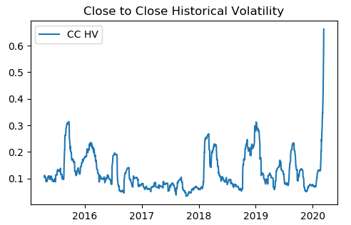
The close-to-close historical volatility (CCHV) is calculated as follows,

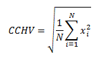
where x_i are the logarithmic returns calculated based on closing prices, and N is the sample size.

The CCHV has the following characteristics

Advantages

It has well-understood sampling properties
It is easy to correct bias
It is easy to convert to a form involving typical daily moves

Disadvantages

It is a very inefficient use of data and converges very slowly

Besides the close-to close historical volatility, we can use other volatility measures. Some of them are described below.

The Parkinson volatility extends the CCHV by incorporating the stock’s daily high and low prices. It is calculated as follow,

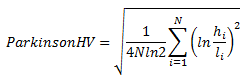
Parkinson volatility analysis in Python

where h_i denotes the daily high price, and l_i is the daily low price.

Garman-Klass volatility estimator uses not only the high and low but also the opening and closing prices. It consists of using the returns of the open, high, low, and closing prices in its calculation. It is calculated as follow,

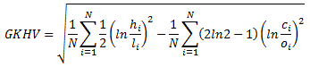
Volatility Analysis in Python Garman-Klass

where h_i denotes the daily high price, l_i is the daily low price, c_i is the daily closing price and o_i is the daily opening price.

Garman-Klass-Yang-Zhang volatility estimator consists of using the returns of open, high, low, and closing prices in its calculation. It also uses the previous day’s closing price. It is calculated as follows,

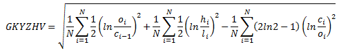
Volatility trading strategy Garman-Klass-Yang-Zhang estimator

where h_i denotes the daily high price, l_i is the daily low price, c_i is the daily closing price and o_i is the daily opening price of the stock at day i.

Risk-free interest rate

Some acceptable sources for risk-free interest rates used in derivative valuation are:

The LIBOR swap rate
Interest rates on direct Treasury obligations of the U.S. government
The Overnight Index Swap rate based on the Fed Funds Effective Rate
The Securities Industry and Financial Markets Association Municipal Swap Rate.

Using the swap rates, a discount factor curve is built by bootstrapping from the short maturity and long maturity in order of increasing maturity. The processes for backing out the discount factors from the short and long maturity swap rates are, however, different.

In the short end of the curve, given that there is only 1 payment, the discount factor is calculated based on the spot rates. At the long end of the curve, the discount factor curve is determined as follows,

Payment dates are generated at each 6 months (or a year, depending on the currency) from the time zero up to 30 years,
Par swap rates are determined at each payment date. To obtain the par swap rates for the payment dates where there are no swap quotes, one linearly interpolates the par swap rates in order to complete the long end of the swap curve,
Using the par swap rates at each payment date, discount factors are obtained by solving a recursive equation.